09/07/15 19:54
To give some practical evidence for the theoretical study about the photon count I exposed the MM2 for 20 seconds with closed lens cap and in the dark. This should ensure that no light would enter the camera. In theory every pixel would have the value = 0. There is an automatically running noise reduction program by Leica (Request: give us the menu option to deselect this option). It is not known what the program does.
The analysis program gives an exact count of every pixel and it can be seen from this selection that the values range from 0 to 12 in this section of the sensor surface. Where there should be zero levels you will find 12 levels, roughly comparable with photons.

This conforms with the random or Poisson noise. Looking at the whole picture I detect four quadrants with equal area, but different noise pattern. See below the section where the four quadrants meet. It is intriguing to see that the top half of the sensor exhibits noise and the lower half almost none. So depending on the area where you look, the noise impression may be different.

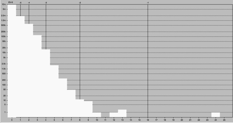
A statistical count of all values gives this graph. Note that there is indeed a heavy concentration of the levels = 0 and = 1, but also quite a lot pixels with higher levels.
Below you find a section of a picture that was overexposed and should show identical pixel values. Note the variation and the fact that some cells exhibit values around 4000. Some persons showed a surprise that the nominal value for maximum white is 3750 and not 4096. The reason is explained in my book Leica Practicum: it is the standard safety level to account for heavy overexposure.

08/07/15 20:10
A CCD and CMOS sensor consists of an array of light detectors that count incoming photons at each location (pixel). The 'count' is in fact the registration of an electric charge that is knocked loose from the semi-conductor material by the incoming light energy. The maximum number of 'counts' is determined by the bit depth of the computer. A 12 bit storage register has a maximum level of 4095 counts/photons and a 14 bit register can count till 16383 photons. The CCD/CMOS sensor reacts linearly to the levels of light energy and doubling the exposure will double the amount of photons (excluding noise and random fluctuations).
The total number of photons that can be counted depends obviously on shutter speed, aperture and sensitivity of sensor. This is analogous to the response of silver-halide crystals in emulsions.
We will approach the issue from two directions: how many photons are available at all in reality (photon flux) and how many photons can a pixel receive before saturation sets in.
In full sun the number of photons reaching the earth is staggering: 3.6 x 10^21 photons per second per square meter. Let us assume that the standard exposure time is 1/60 second. The lux values (classical exposure meter) are: full sun: 80000 and overcast outdoors: 1000.
Because the number of photons is related to the size of the capture area and the exposure time, we need first the area of the pixel in μmeters^2. The area of the pixel of the Leica CMOS sensor is 36 μmeters^2. Dividing the total amount of photons by this value (I used 35 μmeters^2 )and then by 1/60 gives a total of 2.6 x 10^8 for full sun and 3.3 x 10^6 for outdoors overcast. To put these figures in perspective: a star gives 0.33 photons under the same conditions of shutter speed and area.
It seems that there are more than enough photons to saturate even a 16 bit sensor. But now a problem arises. The photons arrive at the pixel in a random fashion. This means that the average number may be constant because it refers to the intensity of the light. What we need however is the probability that the pixel receives a certain number of photons. This probability can be calculated with the help of the Poisson distribution, a statistical tool. When the dynamic range is very small, (2^2) we have only 5 counts, where 0 represents black, 1 equals 1/4 tone, 2 equals 1/2 tone, 3 equals 3/4 tone and 4 equals white. Now let us expect that only 1 photon will hit the surface. The Poisson distribution tells us that for this case the chance of getting 1 photon is about 1/3, but there is also a change of 4% that the pixel will receive 4 photons. The full table is this: 36 % = 0 photons; 36% =1 photon; 18% = 2 photons; 6% = 3 photons; 4% = 4 photons. The Poisson distribution is also valid when the number of expected photons rises, but there is still a variation. When you expect 4 photons there is a 90% change that the actual number will be between 1 and 7. The statistical expectation has to be combined with the standard deviation and then you get the expected relative variation in pixel photon count (or brightness). To give an example: when you expect 20 photons you have a 99.7 % confidence that the actual number of photons will be between 10 and 30 and 68% chance that the number lies between 15 and 25. The more photons you get the more the relative variation becomes lower. But there is another issue! This is shot noise or Poisson noise.
When a pixel gets 16, 17, or 20 photons, the sensor must establish what value is the true mean because only then you get the real value without the noise and the random effects. But the sensor has no way of knowing what this true mean actually is. We need a trick! One way to do it is to group the pixel counts into ranges with boundaries that reflect the limits of the standard deviation (SD). These boundaries represent the confidence limits and are expressed as SD's. If the boundary is set at ± 1 SD, then we may expect with a confidence of 68% that if the photon count falls within a certain partition it is close to the central mean of this partition.
Now the Poisson distribution has the valuable property that its mean equals the square of the standard deviation. If we want that the photon count for the highest photon count for a 16 bit dynamic range is for 99.7% correct (4 SD's!) we have to multiply 65536 (2^16) by 4 and square the result. This produces the unbelievable number of 68,719,476,736 or 2^36 photons that must hit a pixel to be practically certain that the maximum brightness value has been recorded. So many photons are not available at all. For a 14 bit sensor and for a much lower level of certainty (2 SD) the number is still too high: (16384 x 2)^2 = 1.1 x 10^9. Even 14 bit resolution is impossible to reach. A 12 bit resolution is more to the point. Now we can expect 6.7 x 10^7 photons at the maximum brightness level and because we have fixed the SD at 2, the pixel count can actually be within the top brightness range. Remember that all these numbers assume a shutter speed of 1/60. When using higher shutter speeds even less photons will hit the pixel surface and the real dynamic range will be even less.
Conclusion 1: if we wish to exploit the full maximum range of a 16 bit dynamic range the total photon flux in real life is not high enough. A 12 bit dynamic range is much more realistic. With a 16 bit storage register you create an illusion of a very high dynamic range that is impossible to use in real life situations, especially at higher shutter speeds.
To cover all gradations of tonality we want to record we need the range of 1 to 1 million photons per pixel . This range is needed because of the linearity in the dynamic range and to get useable values in the dark areas. This range is not possible to capture even when using a 16 bit resolution that has a maximum brightness value of 65535, much lower than the 1 million that should be covered. This implies that the maximum tonality for perfect imagery can not be reached.
We can also approach the issue from the technical side: the maximum capacity of a pixel (the full well capacity) in modern sensor technology is about 1700 electrons or photons per square micron For the Leica CMOS this amounts to 36 x 1700 = 61200 photons, much more than the possible 4096 values that a 12 bit storage register can handle and much less than the required one million. A bit depth of 16 does not improve the situation much because we still need compression at the maximum brightness side and the electron charge has to be converted to an integer in the range from 32768 to 65535. There are now 32768 brightness steps in the maximum brightness range and it is impossible to differentiate between the brightness steps of say 40023 and 40024.
The 12 bit resolution has a maximum value of 4095. How to relate 60.000 to 4000? The trick is square compression before digitization. One can extract the square root of a number and use that as a replacement. All these calculations assume that all possible photons will indeed be captured by every pixel. Even a 1,4 lens will reduce the number of theoretically possible photons. In reality you may be lucky to get 600 photons in a pixel when not photographing in bright sunlight. The camera hardware will actually amplify this value in the analog domain before it is being converted in the ADC domain with a gain factor.
Conclusion 2: the full well capacity of a typical modern pixel is 1700 photons per square micrometer (micron). The pixel area of the Leica CMOS sensor is ± 36 square micron, so the total number of photons before saturation is about 60000. Leica uses a compression scheme to match the range from 0 - 60000 into the 12 bit dynamic range from 0 - 4095.
Conclusion 3: to get full tonality we need about 1 million photons to cover every possible step in tonality that the human eye can perceive. Because of transmission losses, hardware issues the actual amount may be several million photons. In full sun this is possible, but in less favorable situations the Leica pixel will be able to capture only less than 350000 photons. A higher ISO value does not really help: this only artificially increases the photon count by a gain factor.
Conclusion 4: in low to average brightness levels, at moderate ISO values, with shutter speeds around 1/60 and apertures around 1:2, the actual count may be around 600 photons/pixel. The dynamic level is then artificially increased in the Gain Stage. This is contrary to the working of silver halide where a low density simply implies a low contrast and a low dynamic range.
Final conclusion: the 12 bit resolution of the MM-2 is not a compromise solution but a logical choice given the practical and theoretical issues of photon flux, full well capacity, ADC converter technology and the demands of tonal range and tonal separation.